Blog1: Neural ODE Processes
1 Research problem
Many real-world time series are generated by underlying continuous-time dynamics. Neural Ordinary Differential Equations (Neural ODEs) can model such smooth latent trajectories, but they suffer from two major limitations:
Neural ODEs are unable to adapt to incoming data points, a fundamental requirement for real-time applications imposed by the natural direction of time.
Time series are often composed of a sparse set of measurements that could be explained by many possible underlying dynamics. Neural ODEs do not capture this uncertainty.
Conversely, Neural Processes (NPs) endow models with both adaptation and uncertainty, yet NPs treat inputs as an unordered set and possess no explicit notion of time.
Neural ODE Processes (NDPs) aim to bridge this gap by integrating Neural ODEs with NPs. NDPs define a new class of stochastic processes induced by placing a distribution over Neural ODE initial conditions and/or dynamics.
2 Importance
3 Solution
Mathematically, we aim to learn a random function
\(F: \mathcal{T} \to \mathcal{Y}\),
where \(\mathcal{T} = [t_0, \infty), \quad \mathcal{Y} \subseteq \mathbb{R}^d\)
We assume \(F\) has a distribution \(D\), induced by another distribution \(D'\) over some underlying dynamics that govern the time-series. Given a specific instantation \(\mathcal{F}\) of \(F\), let \(\mathbb{C}={(t_i^{\mathbb{C}},y_i^{\mathbb{C}})}_{i \in I_{\mathbb{C}}}\) be a set of contex points samples from \(\mathcal{F}\) with some indexing set \(I_{\mathbb{C}}\).
For a given context \(\mathbb{C}\), the task is to predict the value \({y_{j}}_{j \in I_{\mathbb{T}}}\) that \(\mathcal{F}\) takes at a set of target times \({t_{j}^{\mathbb{T}}}_{j \in I_{\mathbb{T}}}\), where \(I_{\mathbb{T}}\) is another index set. \(\mathbb{T}={(t_j^{\mathbb{T}},y_j^{\mathbb{T}})}\) is the target set.
3.1 Neural ODEs
Neural ODEs model continuous-time dynamics by using a neural network \(f_θ(z, t)\) to parameterize the instantaneous velocity of a latent state \(z\). Given an initial time \(t_₀\) and a target time \(t_ᵢ\), the framework proceeds in three steps:
Encode the initial observation: \(z(t_0) = h_1(y_0)\).
Evolve the latent state by solving the ODE: \(z(t_i) = z(t_0) + ∫_{t_0}^{t_i} f_θ(z(s), s) ds\)
Decode the output: \(\hat{y}_i = h_2(z(t_i))\).
3.2 Neural Processes
A Neural Process represents one concrete instance of \(F\) by a global latent variable \(z\) that captures the variability of \(F\); thus we have \(F(x_i) = g(x_i, z)\).
For a given context set \(\mathbb{C} = \{(x_i, y_i)\}_{i \in I_{\mathbb{C}}}\) and a target set \(x_{1:n}, y_{1:n}\), the generative process is \[ p(y_{1:n},z|x_{1:n},\mathbb{C}) = p(z|\mathbb{C})\prod_{i=1}^n \mathcal{N}(y_i \mid g(x_i, z), \sigma^2) \]
3.3 Neural ODE Processes (NDPs)
In NDPs, the latent state at a given time is found by evolving a Neural ODE: \[ l(t_i) = l(t_0) + \int_{t_0}^{t_i} f_{\theta}(l(t), d, t) dt \]
where \(f_{\theta}\) is a neural network that models the derivative of the latent state \(l(t)\) with respect to time \(t\). And we allow \(d\) to modulate the derivative of this ODE by acting as a global control signal.
Ultimately, for fixed initial conditions, this results in an uncertainty over the ODE trajectories.
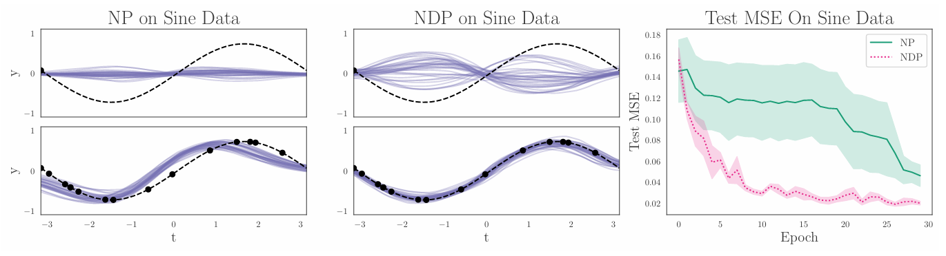
4 Results